Hypothesis Testing

using computer simulation. Based on examples from the infer package. Code for Quiz 13.

Load the R package we will use.

library(tidyverse)
library(infer)
library(skimr)

• Replace all the instances of ???. These are answers on your moodle quiz.

• Run all the individual code chunks to make sure the answers in this file correspond with your quiz answers

• After you check all your code chunks run then you can knit it. It won’t knit until the ??? are replaced

• Save a plot to be your preview plot

Question: t-test

• The data this quiz is a subset of HR
  • Look at the variable definitions
  • Note that the variables evaluation and salary have been recoded to be represented as words instead of numbers
• Set random seed generator to 123

set.seed(123) hr_2_tidy.csv is the name of your data subset

• Read it into and assign to hr_anova

  • Note: col_types = “fddfff” defines the column types factor-double-double-factor-factor-factor

hr  <- read_csv("https://estanny.com/static/week13/data/hr_2_tidy.csv", 
                col_types = "fddfff")

use the skim to summarize the data in hr

skim(hr)

Table 1: Data summary

Name	hr
Number of rows	500
Number of columns	6
_______________________
Column type frequency:
factor	4
numeric	2
________________________
Group variables	None

Variable type: factor

skim_variable	n_missing	complete_rate	ordered	n_unique	top_counts
gender	0	1	FALSE	2	mal: 256, fem: 244
evaluation	0	1	FALSE	4	bad: 154, fai: 142, goo: 108, ver: 96
salary	0	1	FALSE	6	lev: 95, lev: 94, lev: 87, lev: 85
status	0	1	FALSE	3	fir: 194, pro: 179, ok: 127

Variable type: numeric

skim_variable	n_missing	complete_rate	mean	sd	p0	p25	p50	p75	p100	hist
age	0	1	39.86	11.55	20.3	29.60	40.2	50.1	59.9	▇▇▇▇▇
hours	0	1	49.39	13.15	35.0	37.48	45.6	58.9	79.9	▇▃▂▂▂

The mean hours worked per week is: 49.4

Q: Is the mean number of hours worked per week 48?

specify that hours is the variable of interest

hr  %>% 
  specify(response = hours)

Response: hours (numeric)
# A tibble: 500 x 1
   hours
   <dbl>
 1  78.1
 2  35.1
 3  36.9
 4  38.5
 5  36.1
 6  78.1
 7  76  
 8  35.6
 9  35.6
10  56.8
# ... with 490 more rows

hypothesize that the average hours worked is 48

hr  %>% 
  specify(response = hours)  %>% 
  hypothesize(null = "point", mu = 48)

Response: hours (numeric)
Null Hypothesis: point
# A tibble: 500 x 1
   hours
   <dbl>
 1  78.1
 2  35.1
 3  36.9
 4  38.5
 5  36.1
 6  78.1
 7  76  
 8  35.6
 9  35.6
10  56.8
# ... with 490 more rows

generate 1000 replicates representing the null hypothesis

hr %>% 
  specify(response = hours)  %>% 
  hypothesize(null = "point", mu = 48)  %>% 
  generate(reps = 1000, type = "bootstrap")

Response: hours (numeric)
Null Hypothesis: point
# A tibble: 500,000 x 2
# Groups:   replicate [1,000]
   replicate hours
       <int> <dbl>
 1         1  34.7
 2         1  70.1
 3         1  45.6
 4         1  42.9
 5         1  48.3
 6         1  47.0
 7         1  43.3
 8         1  56.1
 9         1  45.8
10         1  33.8
# ... with 499,990 more rows

• calculate the distribution of statistics from the generated data

  • Assign the output null_t_distribution

  • Display null_t_distribution

null_t_distribution  <- hr  %>% 
  specify(response = age)  %>% 
  hypothesize(null = "point", mu = 48)  %>% 
  generate(reps = 1000, type = "bootstrap")  %>% 
  calculate(stat = "t")

null_t_distribution

# A tibble: 1,000 x 2
   replicate    stat
 *     <int>   <dbl>
 1         1  1.82  
 2         2  0.334 
 3         3  1.98  
 4         4 -0.568 
 5         5  0.595 
 6         6  0.725 
 7         7  1.15  
 8         8 -0.423 
 9         9 -1.22  
10        10 -0.0591
# ... with 990 more rows

null_t_distribution has 1000 t-stats

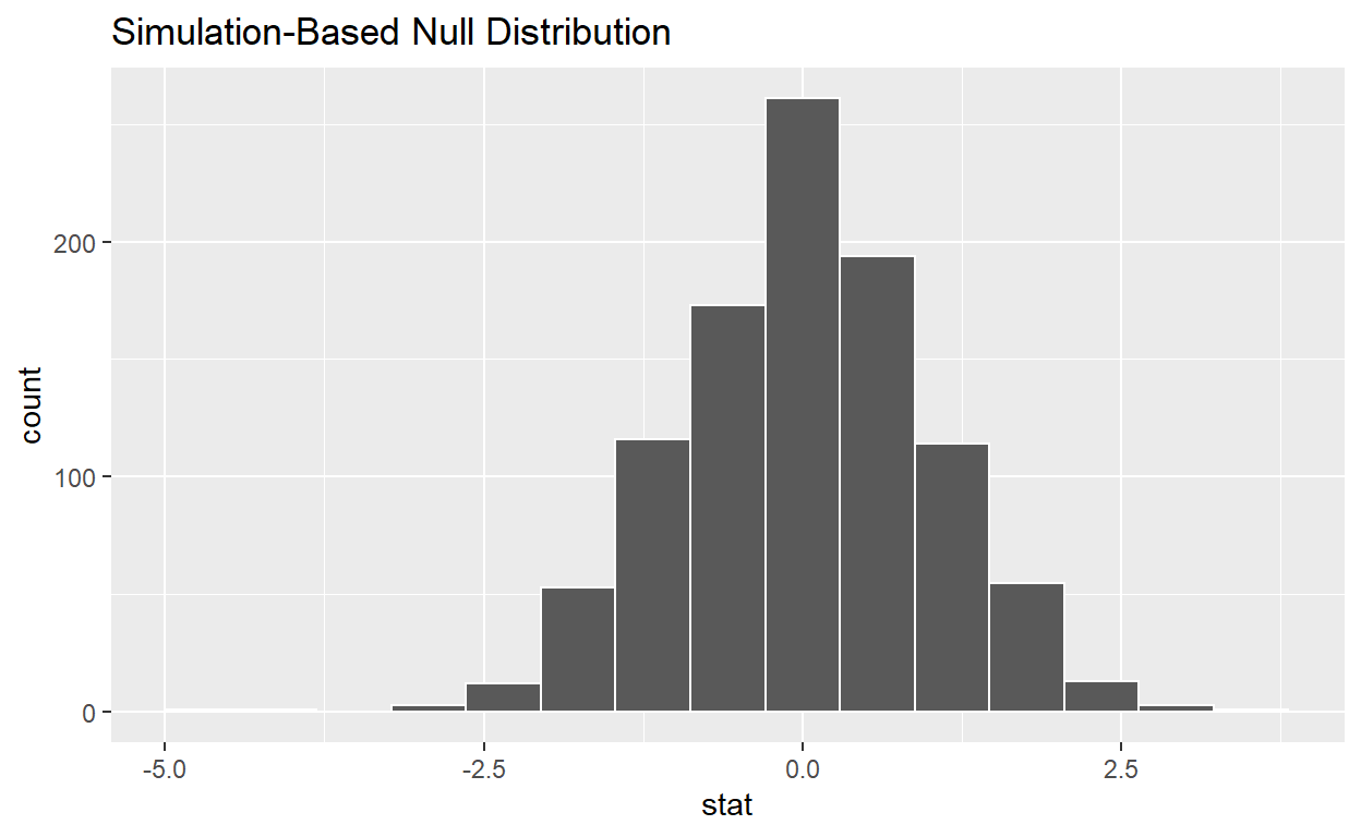
visualize the simulated null distribution

visualize(null_t_distribution)

calculate the statistic from your observed data

• Assign the output observed_t_statistic

• Display observed_t_statistic

observed_t_statistic  <- hr  %>%
  specify(response = hours)  %>% 
  hypothesize(null = "point", mu = 48)  %>%
  calculate(stat = "t")

observed_t_statistic

# A tibble: 1 x 1
   stat
  <dbl>
1  2.37

get_p_value from the simulated null distribution and the observed statistic

null_t_distribution  %>% 
  get_p_value(obs_stat = observed_t_statistic , direction = "two-sided")

# A tibble: 1 x 1
  p_value
    <dbl>
1   0.014

shade_p_value on the simulated null distribution

null_t_distribution  %>% 
  visualize() +
  shade_p_value(obs_stat = observed_t_statistic, direction = "two-sided")

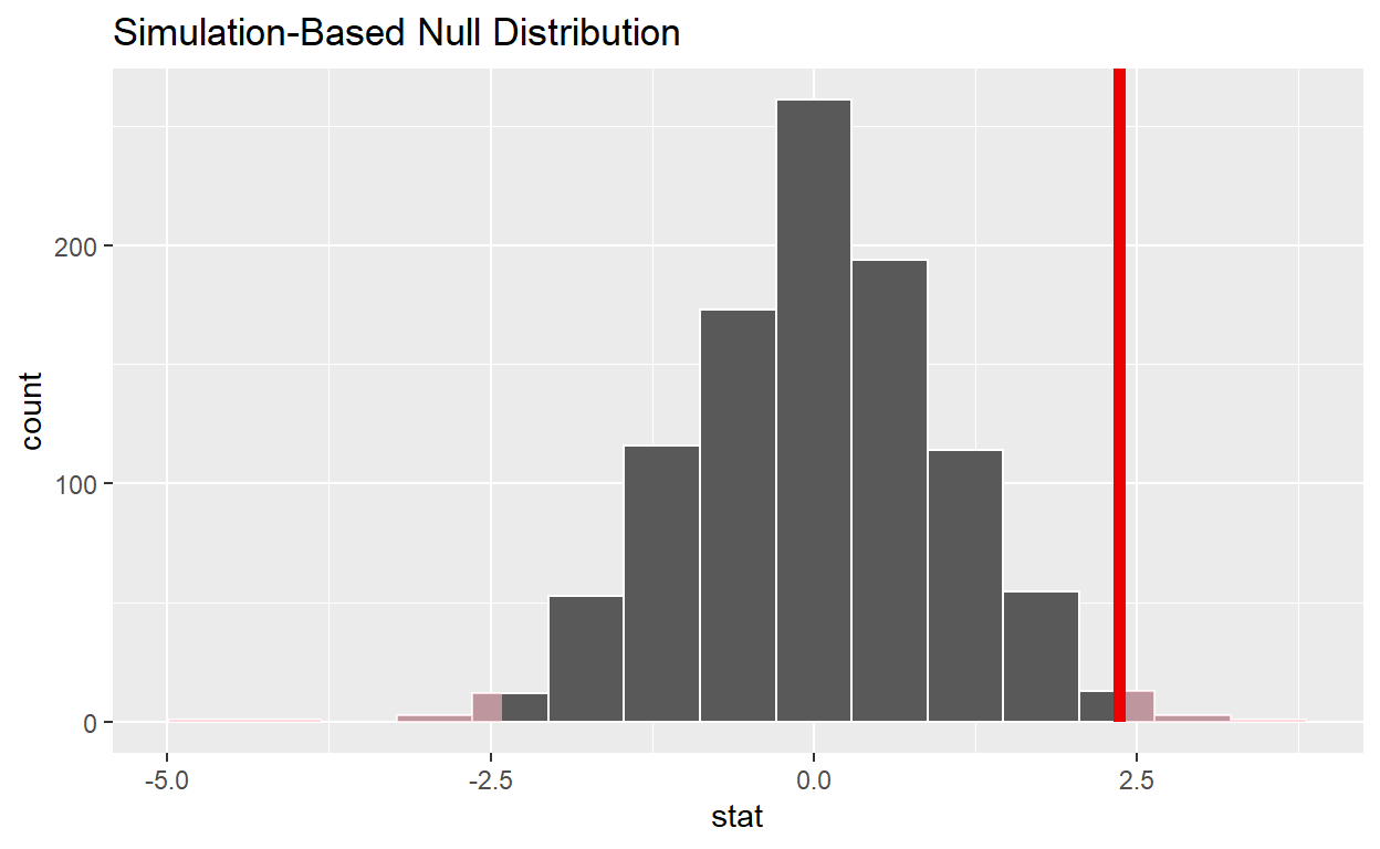
If the p-value < 0.05? yes (yes/no)

Does your analysis support the null hypothesis that the true mean number of hours worked was 48? no (yes/no)

Question: 2 sample t-test

hr_3_tidy.csv is the name of your data subset

• Read it into and assign to hr_2

  • Note: col_types = “fddfff” defines the column types factor-double-double-factor-factor-factor

hr_2 <- read_csv("https://estanny.com/static/week13/data/hr_3_tidy.csv", 
                col_types = "fddfff")

Q: Is the average number of hours worked the same for both genders in hr_2?

use skim to summarize the data in hr_2 by gender

hr_2 %>% 
  group_by(gender)  %>% 
  skim()

Table 2: Data summary

Name	Piped data
Number of rows	500
Number of columns	6
_______________________
Column type frequency:
factor	3
numeric	2
________________________
Group variables	gender

Variable type: factor

skim_variable	gender	n_missing	complete_rate	ordered	n_unique	top_counts
evaluation	male	0	1	FALSE	4	bad: 72, fai: 67, goo: 61, ver: 47
evaluation	female	0	1	FALSE	4	bad: 76, fai: 71, goo: 61, ver: 45
salary	male	0	1	FALSE	6	lev: 47, lev: 43, lev: 43, lev: 42
salary	female	0	1	FALSE	6	lev: 51, lev: 46, lev: 45, lev: 43
status	male	0	1	FALSE	3	fir: 98, pro: 81, ok: 68
status	female	0	1	FALSE	3	fir: 98, pro: 91, ok: 64

Variable type: numeric

skim_variable	gender	n_missing	complete_rate	mean	sd	p0	p25	p50	p75	p100	hist
age	male	0	1	38.23	10.86	20	28.9	37.9	47.05	59.9	▇▇▇▇▅
age	female	0	1	40.56	11.67	20	31.0	40.3	50.50	59.8	▆▆▇▆▇
hours	male	0	1	49.55	13.11	35	38.4	45.4	57.65	79.9	▇▃▂▂▂
hours	female	0	1	49.80	13.38	35	38.2	45.6	59.40	79.8	▇▂▃▂▂

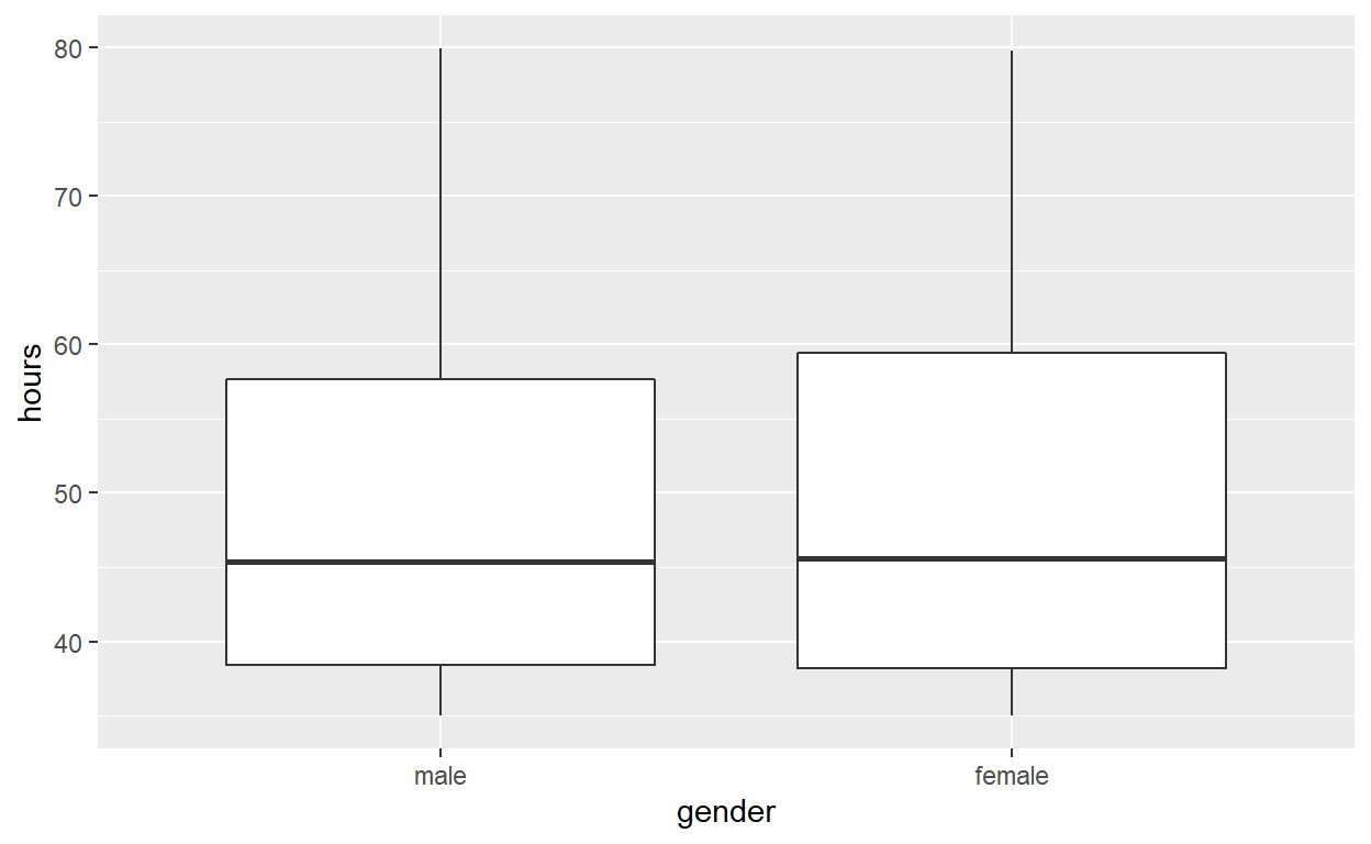
Use geom_boxplot to plot distributions of hours worked by gender

hr_2 %>% 
  ggplot(aes(x = gender, y = hours)) + 
  geom_boxplot()

specify the variables of interest are hours and gender

hr_2 %>% 
  specify(response = hours, explanatory = gender)

Response: hours (numeric)
Explanatory: gender (factor)
# A tibble: 500 x 2
   hours gender
   <dbl> <fct> 
 1  49.6 male  
 2  39.2 female
 3  63.2 female
 4  42.2 male  
 5  54.7 male  
 6  54.3 female
 7  37.3 female
 8  45.6 female
 9  35.1 female
10  53   male  
# ... with 490 more rows

hypothesize that the number of hours worked and gender are independent

hr_2  %>% 
  specify(response = hours, explanatory = gender)  %>% 
  hypothesize(null = "independence")

Response: hours (numeric)
Explanatory: gender (factor)
Null Hypothesis: independence
# A tibble: 500 x 2
   hours gender
   <dbl> <fct> 
 1  49.6 male  
 2  39.2 female
 3  63.2 female
 4  42.2 male  
 5  54.7 male  
 6  54.3 female
 7  37.3 female
 8  45.6 female
 9  35.1 female
10  53   male  
# ... with 490 more rows

generate 1000 replicates representing the null hypothesis

hr_2 %>% 
  specify(response = hours, explanatory = gender)  %>% 
  hypothesize(null = "independence")  %>% 
  generate(reps = 1000, type = "permute") 

Response: hours (numeric)
Explanatory: gender (factor)
Null Hypothesis: independence
# A tibble: 500,000 x 3
# Groups:   replicate [1,000]
   hours gender replicate
   <dbl> <fct>      <int>
 1  56.8 male           1
 2  66.1 female         1
 3  42.5 female         1
 4  48.5 male           1
 5  37.4 male           1
 6  37   female         1
 7  71.9 female         1
 8  56.5 female         1
 9  35.1 female         1
10  66.4 male           1
# ... with 499,990 more rows

calculate the distribution of statistics from the generated data

• Assign the output null_distribution_2_sample_permute

• Display null_distribution_2_sample_permute

null_distribution_2_sample_permute  <- hr_2 %>% 
  specify(response = hours, explanatory = gender)  %>% 
  hypothesize(null = "independence")  %>% 
  generate(reps = 1000, type = "permute")  %>% 
  calculate(stat = "t", order = c("female", "male"))

null_distribution_2_sample_permute

# A tibble: 1,000 x 2
   replicate    stat
 *     <int>   <dbl>
 1         1  1.97  
 2         2  0.983 
 3         3 -1.49  
 4         4  0.568 
 5         5 -0.496 
 6         6 -0.644 
 7         7  1.83  
 8         8 -0.0292
 9         9 -0.615 
10        10  0.529 
# ... with 990 more rows

null_t_distribution has 1000 t-stats

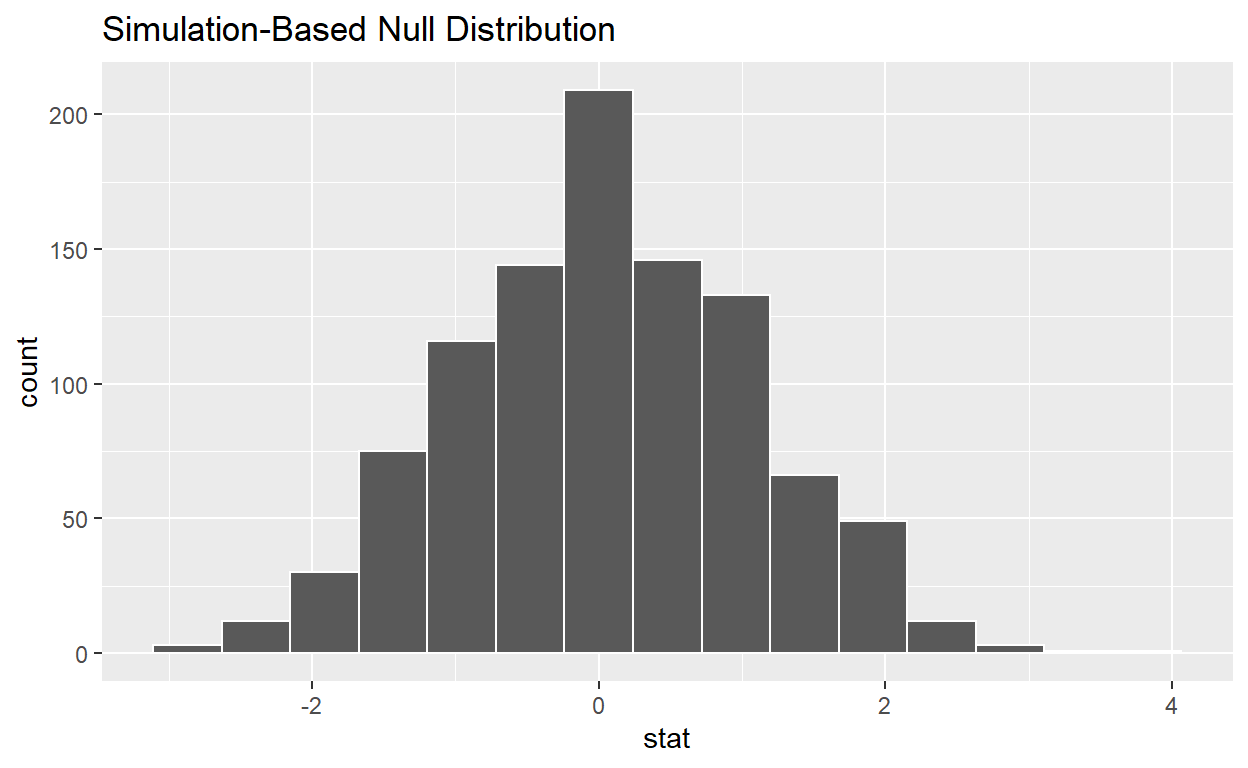
visualize the simulated null distribution

visualize(null_distribution_2_sample_permute)

calculate the statistic from your observed data

• Assign the output observed_t_2_sample_stat

• Display observed_t_2_sample_stat

observed_t_2_sample_stat  <- hr_2 %>%
  specify(response = hours, explanatory = gender)  %>% 
  calculate(stat = "t", order = c("female", "male"))

observed_t_2_sample_stat

# A tibble: 1 x 1
   stat
  <dbl>
1 0.208

get_p_value from the simulated null distribution and the observed statistic

null_t_distribution  %>% 
  get_p_value(obs_stat = observed_t_2_sample_stat , direction = "two-sided")

# A tibble: 1 x 1
  p_value
    <dbl>
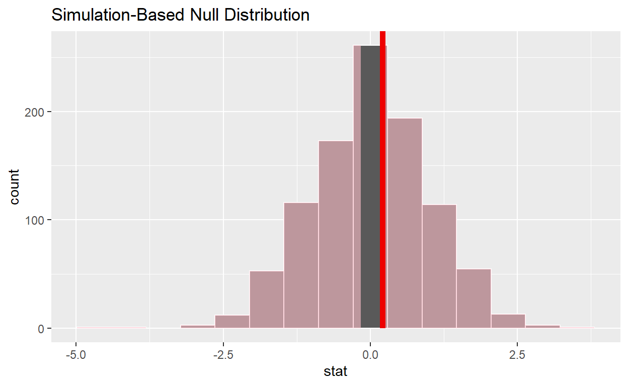
1   0.826

shade_p_value on the simulated null distribution

null_t_distribution  %>% 
  visualize() +
  shade_p_value(obs_stat = observed_t_2_sample_stat, direction = "two-sided")

ggsave(filename = "preview.png", 
       path = here::here("_posts", "2021-05-05-hypothesis-testing"))

If the p-value < 0.05? no (yes/no)

Does your analysis support the null hypothesis that the true mean number of hours worked by female and male employees was the same? yes (yes/no)

Question: ANOVA

hr_3_tidy.csv is the name of your data subset

• Read it into and assign to hr_anova

  • Note: col_types = “fddfff” defines the column types factor-double-double-factor-factor-factor

hr_anova <- read_csv("https://estanny.com/static/week13/data/hr_3_tidy.csv", 
                col_types = "fddfff")

Q: Is the average number of hours worked the same for all three status (fired, ok and promoted) ?

use skim to summarize the data in hr_anova by status

hr_anova %>% 
  group_by(status)  %>% 
  skim()

Table 3: Data summary

Name	Piped data
Number of rows	500
Number of columns	6
_______________________
Column type frequency:
factor	3
numeric	2
________________________
Group variables	status

Variable type: factor

skim_variable	status	n_missing	complete_rate	ordered	n_unique	top_counts
gender	promoted	0	1	FALSE	2	fem: 91, mal: 81
gender	fired	0	1	FALSE	2	mal: 98, fem: 98
gender	ok	0	1	FALSE	2	mal: 68, fem: 64
evaluation	promoted	0	1	FALSE	4	goo: 79, ver: 52, fai: 21, bad: 20
evaluation	fired	0	1	FALSE	4	bad: 77, fai: 64, ver: 30, goo: 25
evaluation	ok	0	1	FALSE	4	fai: 53, bad: 51, goo: 18, ver: 10
salary	promoted	0	1	FALSE	6	lev: 42, lev: 37, lev: 36, lev: 28
salary	fired	0	1	FALSE	6	lev: 59, lev: 40, lev: 39, lev: 25
salary	ok	0	1	FALSE	6	lev: 33, lev: 29, lev: 28, lev: 23

Variable type: numeric

skim_variable	status	n_missing	complete_rate	mean	sd	p0	p25	p50	p75	p100	hist
age	promoted	0	1	40.22	11.11	20.1	31.67	41.00	48.82	59.7	▆▇▇▇▇
age	fired	0	1	38.95	11.23	20.0	29.82	38.80	48.75	59.9	▇▆▇▇▅
age	ok	0	1	39.03	11.77	20.0	28.28	38.75	49.92	59.7	▇▇▆▇▆
hours	promoted	0	1	59.29	12.53	35.0	49.90	58.65	70.35	79.9	▅▆▇▆▇
hours	fired	0	1	42.37	9.15	35.0	36.20	39.20	43.80	79.6	▇▁▁▁▁
hours	ok	0	1	47.99	11.55	35.0	37.45	45.75	55.23	75.7	▇▃▃▂▂

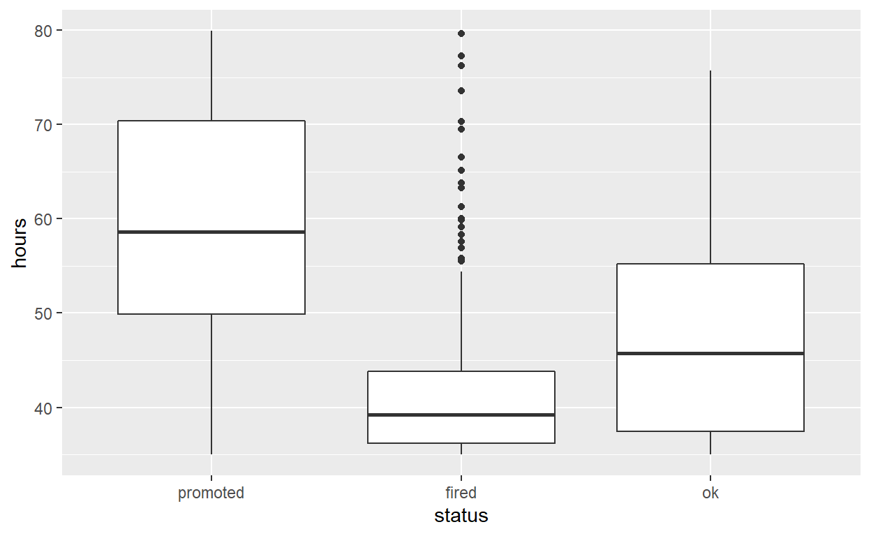
• Employees that were fired worked an average of 42.4 hours per week

• Employees that were ok worked an average of 48.0 hours per week

• Employees that were promoted worked an average of 59.3 hours per week

Use geom_boxplot to plot distributions of hours worked by status

hr_anova %>% 
  ggplot(aes(x = status, y = hours)) + 
  geom_boxplot()

specify the variables of interest are hours and status

hr_anova %>% 
  specify(response = hours, explanatory = status)

Response: hours (numeric)
Explanatory: status (factor)
# A tibble: 500 x 2
   hours status  
   <dbl> <fct>   
 1  49.6 promoted
 2  39.2 fired   
 3  63.2 promoted
 4  42.2 promoted
 5  54.7 promoted
 6  54.3 fired   
 7  37.3 fired   
 8  45.6 promoted
 9  35.1 fired   
10  53   promoted
# ... with 490 more rows

hypothesize that the number of hours worked and status are independent

hr_anova  %>% 
  specify(response = hours, explanatory = status)  %>% 
  hypothesize(null = "independence")

Response: hours (numeric)
Explanatory: status (factor)
Null Hypothesis: independence
# A tibble: 500 x 2
   hours status  
   <dbl> <fct>   
 1  49.6 promoted
 2  39.2 fired   
 3  63.2 promoted
 4  42.2 promoted
 5  54.7 promoted
 6  54.3 fired   
 7  37.3 fired   
 8  45.6 promoted
 9  35.1 fired   
10  53   promoted
# ... with 490 more rows

generate 1000 replicates representing the null hypothesis

hr_anova %>% 
  specify(response = hours, explanatory = status)  %>% 
  hypothesize(null = "independence")  %>% 
  generate(reps = 1000, type = "permute")

Response: hours (numeric)
Explanatory: status (factor)
Null Hypothesis: independence
# A tibble: 500,000 x 3
# Groups:   replicate [1,000]
   hours status   replicate
   <dbl> <fct>        <int>
 1  56.5 promoted         1
 2  35.3 fired            1
 3  70.3 promoted         1
 4  35.4 promoted         1
 5  36.6 promoted         1
 6  47.7 fired            1
 7  42.2 fired            1
 8  79.7 promoted         1
 9  70.7 fired            1
10  44   promoted         1
# ... with 499,990 more rows

The output has 500000 rows

calculate the distribution of statistics from the generated data

• Assign the output null_distribution_anova

• Display null_distribution_anova

null_distribution_anova  <- hr_anova %>% 
  specify(response = hours, explanatory = gender)  %>% 
  hypothesize(null = "independence")  %>% 
  generate(reps = 1000, type = "permute")  %>% 
  calculate(stat = "F")

null_distribution_anova

# A tibble: 1,000 x 2
   replicate    stat
 *     <int>   <dbl>
 1         1 0.364  
 2         2 2.04   
 3         3 0.0339 
 4         4 3.32   
 5         5 0.0212 
 6         6 0.331  
 7         7 1.13   
 8         8 0.298  
 9         9 0.847  
10        10 0.00505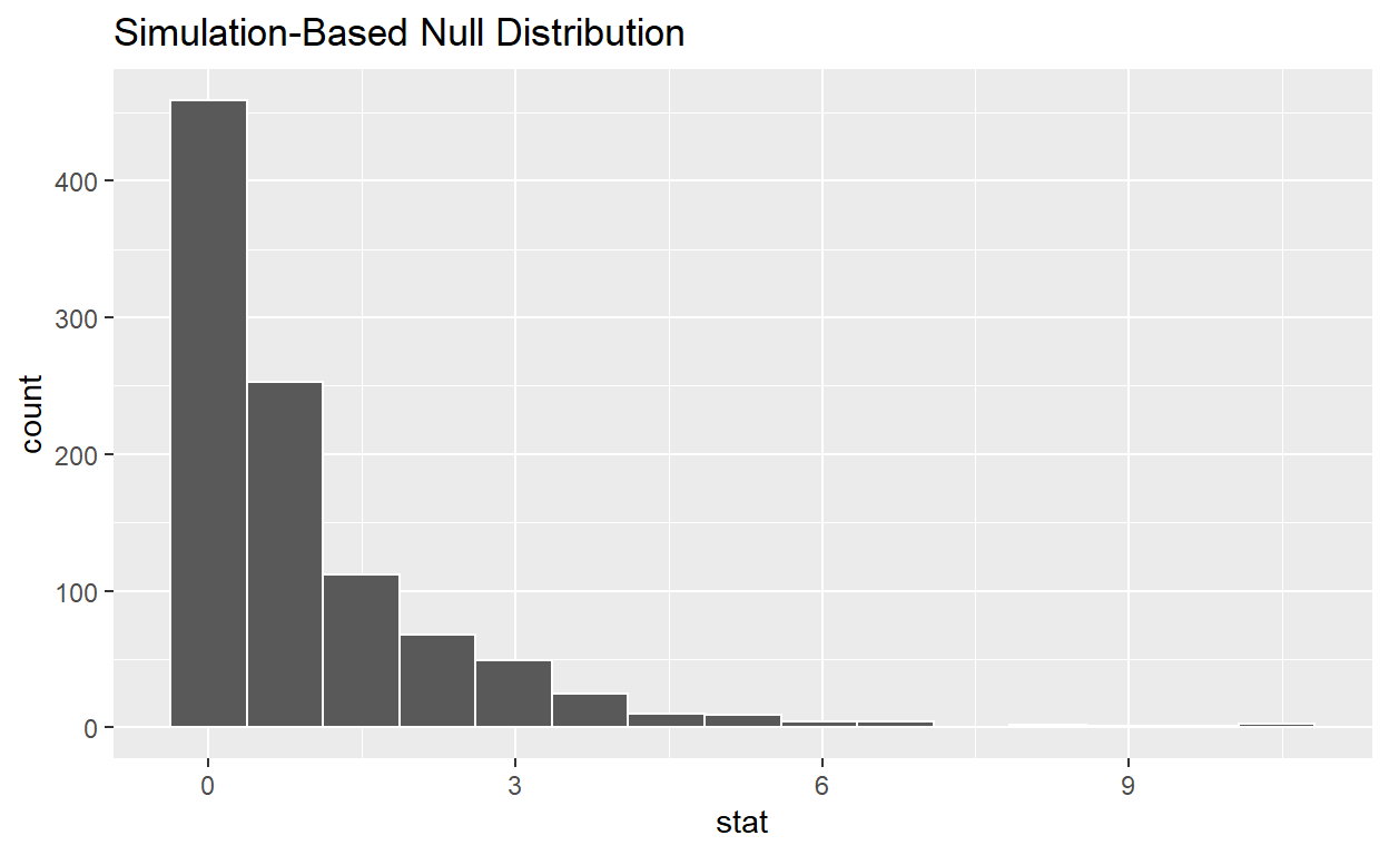
# ... with 990 more rows

• null_distribution_anova has 1000 F-stats visualize the simulated null distribution

visualize(null_distribution_anova)

calculate the statistic from your observed data

• Assign the output observed_f_sample_stat

• Display observed_f_sample_stat

observed_f_sample_stat  <- hr_anova %>%
  specify(response = hours, explanatory = status)  %>% 
  calculate(stat = "F")

observed_f_sample_stat

# A tibble: 1 x 1
   stat
  <dbl>
1  110.

get_p_value from the simulated null distribution and the observed statistic

null_distribution_anova  %>% 
  get_p_value(obs_stat = observed_f_sample_stat , direction = "greater")

# A tibble: 1 x 1
  p_value
    <dbl>
1       0

shade_p_value on the simulated null distribution

null_t_distribution  %>% 
  visualize() +
  shade_p_value(obs_stat = observed_f_sample_stat, direction = "greater")

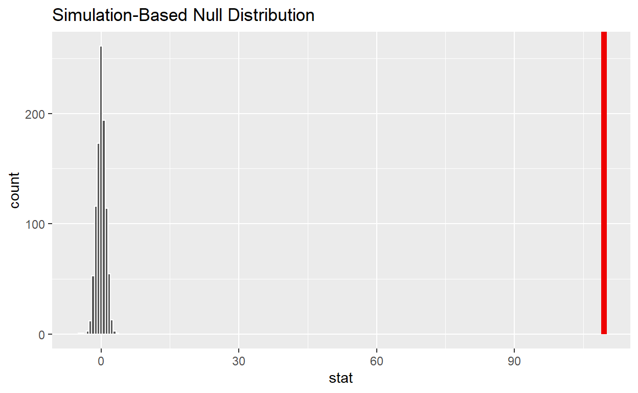
If the p-value < 0.05? yes (yes/no)

Does your analysis support the null hypothesis that the true means of the number of hours worked for those that were “fired”, “ok” and “promoted” were the same? no (yes/no)